Alpha Shape Toolbox


Toolbox for generating n-dimensional alpha shapes.
Alpha shapes are often used to generalize bounding polygons containing sets of points. The alpha parameter is defined as the value a, such that an edge of a disk of radius 1/a can be drawn between any two edge members of a set of points and still contain all the points. The convex hull, a shape resembling what you would see if you wrapped a rubber band around pegs at all the data points, is an alpha shape where the alpha parameter is equal to zero. In this toolbox we will be generating alpha complexes, which are closely related to alpha shapes, but which consist of straight lines between the edge points instead of arcs of circles.
https://en.wikipedia.org/wiki/Alpha_shape
https://en.wikipedia.org/wiki/Convex_hull
Creating alpha shapes around sets of points usually requires a visually interactive step where the alpha parameter for a concave hull is determined by iterating over or bisecting values to approach a best fit. The alpha shape toolbox provides workflows to shorten the development loop on this manual process, or to bypass it completely by solving for an alpha shape with particular characteristics. A python API is provided to aid in the scripted generation of alpha shapes. A console application is also provided as an example usage of the alpha shape toolbox, and to facilitate generation of alpha shapes from the command line.
Free software: MIT license
Documentation: https://alphashape.readthedocs.io.
Features
Import Dependencies
import os
import sys
import pandas as pd
import numpy as np
from descartes import PolygonPatch
import matplotlib.pyplot as plt
sys.path.insert(0, os.path.dirname(os.getcwd()))
import alphashape
2 Dimensional Example
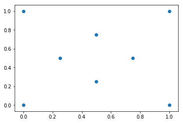
Define a set of points
points_2d = [(0., 0.), (0., 1.), (1., 1.), (1., 0.),
          (0.5, 0.25), (0.5, 0.75), (0.25, 0.5), (0.75, 0.5)]
Visualize Test Coordinates
fig, ax = plt.subplots()
ax.scatter(*zip(*points_2d))
plt.show()
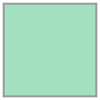
Generate an Alpha Shape ($alpha=0.0$) (Convex Hull)
Every convex hull is an alpha shape, but not every alpha shape is a convex hull. When the alphashape function is called with an alpha parameter of 0, a convex hull will always be returned.
Create the alpha shape
You can visualize the shape within Jupyter notebooks using the built-in shapely renderer as shown below.
alpha_shape = alphashape.alphashape(points_2d, 0.)
alpha_shape
Plotting the alpha shape over the input data with Matplotlib
fig, ax = plt.subplots()
ax.scatter(*zip(*points_2d))
ax.add_patch(PolygonPatch(alpha_shape, alpha=0.2))
plt.show()
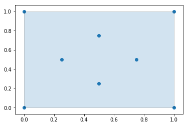
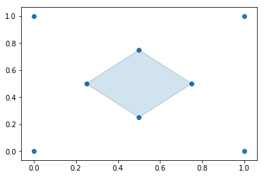
Generate an Alpha Shape ($alpha=2.0$) (Concave Hull)
As we increase the alpha parameter value, the bounding shape will begin to fit the sample data with a more tightly fitting bounding box.
Create the alpha shape
alpha_shape = alphashape.alphashape(points_2d, 2.0)
alpha_shape

Plotting the alpha shape over the input data with Matplotlib
fig, ax = plt.subplots()
ax.scatter(*zip(*points_2d))
ax.add_patch(PolygonPatch(alpha_shape, alpha=0.2))
plt.show()
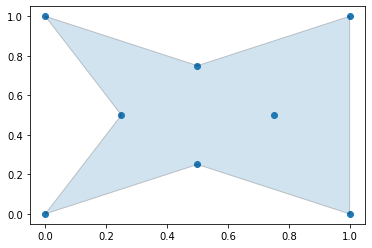
Generate an Alpha Shape ($alpha=3.5$)
If you go too high on the alpha parameter, you will start to lose points from the original data set.
Create the alpha shape
alpha_shape = alphashape.alphashape(points_2d, 3.5)
alpha_shape

Plotting the alpha shape over the input data with Matplotlib
fig, ax = plt.subplots()
ax.scatter(*zip(*points_2d))
ax.add_patch(PolygonPatch(alpha_shape, alpha=0.2))
plt.show()
Generate an Alpha Shape (Alpha=5.0)
If you go too far, you will lose everything.
alpha_shape = alphashape.alphashape(points_2d, 5.0)
print(alpha_shape)
GEOMETRYCOLLECTION EMPTY
Using a varying Alpha Parameter
The alpha parameter can be defined locally within a region of points by supplying a callback that will return what alpha parameter to use. This can be utilized to create tighter fitting alpha shapes where point densitities are different in different regions of a data set. In the following example, the alpha parameter is changed based off of the value of the x-coordinate of the points.
alpha_shape = alphashape.alphashape(
    points_2d,
    lambda ind, r: 1.0 + any(np.array(points_2d)[ind][:,0] == 0.0))
alpha_shape

fig, ax = plt.subplots()
ax.scatter(*zip(*points_2d))
ax.add_patch(PolygonPatch(alpha_shape, alpha=0.2))
plt.show()
The alpha parameter can be solved for if it is not provided as an argument, but with large datasets this can take a long time to calculate.
alpha_shape = alphashape.alphashape(points_2d)
alpha_shape
fig, ax = plt.subplots()
ax.scatter(*zip(*points_2d))
ax.add_patch(PolygonPatch(alpha_shape, alpha=0.2))
plt.show()

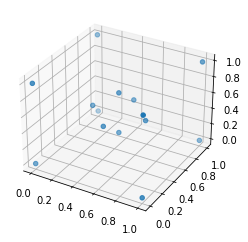
3 Dimensional Example
Define a set of points
points_3d = [
    (0., 0., 0.), (0., 0., 1.), (0., 1., 0.),
    (1., 0., 0.), (1., 1., 0.), (1., 0., 1.),
    (0., 1., 1.), (1., 1., 1.), (.25, .5, .5),
    (.5, .25, .5), (.5, .5, .25), (.75, .5, .5),
    (.5, .75, .5), (.5, .5, .75)
]
Visualize Test Coordinates
fig = plt.figure()
ax = plt.axes(projection='3d')
ax.scatter(df_3d['x'], df_3d['y'], df_3d['z'])
plt.show()
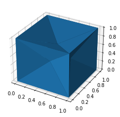
Alphashape with Static Alpha Parameter
You can visualize the shape within Jupyter notebooks using the built-in trimesh renderer by calling the .show() method as shown below.
alpha_shape = alphashape.alphashape(points_3d, 1.1)
alpha_shape.show()
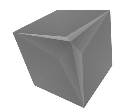
fig = plt.figure()
ax = plt.axes(projection='3d')
ax.plot_trisurf(*zip(*alpha_shape.vertices), triangles=alpha_shape.faces)
plt.show()
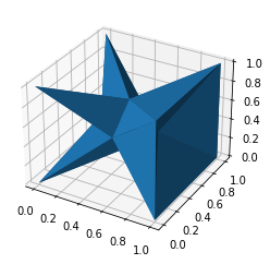
Alphashape with Dymanic Alpha Parameter
alpha_shape = alphashape.alphashape(points_3d, lambda ind, r: 1.0 + any(
    np.array(points_3d)[ind][:,0] == 0.0))
alpha_shape.show()

fig = plt.figure()
ax = plt.axes(projection='3d')
ax.plot_trisurf(*zip(*alpha_shape.vertices), triangles=alpha_shape.faces)
plt.show()
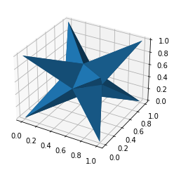
Alphashape found by solving for the Alpha Parameter
alpha_shape = alphashape.alphashape(points_3d)
alpha_shape.show()

fig = plt.figure()
ax = plt.axes(projection='3d')
ax.plot_trisurf(*zip(*alpha_shape.vertices), triangles=alpha_shape.faces)
plt.show()
4 Dimensional Example
Define a set of points
points_4d = [
    (0., 0., 0., 0.), (0., 0., 0., 1.), (0., 0., 1., 0.),
    (0., 1., 0., 0.), (0., 1., 1., 0.), (0., 1., 0., 1.),
    (0., 0., 1., 1.), (0., 1., 1., 1.), (1., 0., 0., 0.),
    (1., 0., 0., 1.), (1., 0., 1., 0.), (1., 1., 0., 0.),
    (1., 1., 1., 0.), (1., 1., 0., 1.), (1., 0., 1., 1.),
    (1., 1., 1., 1.), (.25, .5, .5, .5), (.5, .25, .5, .5),
    (.5, .5, .25, .5), (.5, .5, .5, .25), (.75, .5, .5, .5),
    (.5, .75, .5, .5), (.5, .5, .75, .5), (.5, .5, .5, .75)
]
df_4d = pd.DataFrame(points_4d, columns=['x', 'y', 'z', 'r'])
Visualize Test Coordinates
fig = plt.figure()
ax = plt.axes(projection='3d')
ax.scatter(df_4d['x'], df_4d['y'], df_4d['z'], c=df_4d['r'])
plt.show()

The Edges of a 4 Dimensional Alpha Shape are Tetrahedrons Defined by the Following Coordinates (No Visualizations)
alphashape.alphashape(points_4d, 1.0)
{(16, 1, 2, 0),
 (16, 1, 3, 0),
 (16, 2, 3, 0),
 (16, 4, 2, 3),
 (16, 4, 7, 2),
 (16, 4, 7, 3),
 (16, 5, 1, 3),
 (16, 5, 7, 1),
 (16, 5, 7, 3),
 (16, 6, 1, 2),
 (16, 6, 7, 1),
 (16, 6, 7, 2),
 (17, 1, 2, 0),
 (17, 1, 8, 0),
 (17, 2, 8, 0),
 (17, 6, 1, 2),
 (17, 6, 14, 1),
 (17, 6, 14, 2),
 (17, 9, 1, 8),
 (17, 9, 14, 1),
 (17, 9, 14, 8),
 (17, 10, 2, 8),
 (17, 10, 14, 2),
 (17, 10, 14, 8),
 (18, 1, 3, 0),
 (18, 1, 8, 0),
 (18, 3, 8, 0),
 (18, 5, 1, 3),
 (18, 5, 13, 1),
 (18, 5, 13, 3),
 (18, 9, 1, 8),
 (18, 9, 13, 1),
 (18, 9, 13, 8),
 (18, 11, 3, 8),
 (18, 11, 13, 3),
 (18, 11, 13, 8),
 (19, 2, 3, 0),
 (19, 2, 8, 0),
 (19, 3, 8, 0),
 (19, 4, 2, 3),
 (19, 4, 12, 2),
 (19, 4, 12, 3),
 (19, 10, 2, 8),
 (19, 10, 12, 2),
 (19, 10, 12, 8),
 (19, 11, 3, 8),
 (19, 11, 12, 3),
 (19, 11, 12, 8),
 (20, 9, 13, 8),
 (20, 9, 14, 8),
 (20, 9, 14, 13),
 (20, 10, 12, 8),
 (20, 10, 14, 8),
 (20, 10, 14, 12),
 (20, 11, 12, 8),
 (20, 11, 13, 8),
 (20, 11, 13, 12),
 (20, 13, 12, 15),
 (20, 14, 12, 15),
 (20, 14, 13, 15),
 (21, 4, 7, 3),
 (21, 4, 7, 12),
 (21, 4, 12, 3),
 (21, 5, 7, 3),
 (21, 5, 7, 13),
 (21, 5, 13, 3),
 (21, 7, 12, 15),
 (21, 7, 13, 15),
 (21, 11, 12, 3),
 (21, 11, 13, 3),
 (21, 11, 13, 12),
 (21, 13, 12, 15),
 (22, 4, 7, 2),
 (22, 4, 7, 12),
 (22, 4, 12, 2),
 (22, 6, 7, 2),
 (22, 6, 7, 14),
 (22, 6, 14, 2),
 (22, 7, 12, 15),
 (22, 7, 14, 15),
 (22, 10, 12, 2),
 (22, 10, 14, 2),
 (22, 10, 14, 12),
 (22, 14, 12, 15),
 (23, 5, 7, 1),
 (23, 5, 7, 13),
 (23, 5, 13, 1),
 (23, 6, 7, 1),
 (23, 6, 7, 14),
 (23, 6, 14, 1),
 (23, 7, 13, 15),
 (23, 7, 14, 15),
 (23, 9, 13, 1),
 (23, 9, 14, 1),
 (23, 9, 14, 13),
 (23, 14, 13, 15)}
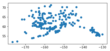
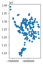
Alpha Shapes with GeoPandas
The data used in this notebook can be obtained from the Alaska Department of Transportation and Public Facilities website at the link below. It consists of a point collection for each of the public airports in Alaska.
http://www.dot.alaska.gov/stwdplng/mapping/shapefiles.shtml
import os
import geopandas
data = os.path.join(os.getcwd(), 'data', 'Public_Airports_March2018.shp')
gdf = geopandas.read_file(data)
%matplotlib inline
gdf.plot()
gdf.crs
{'init': 'epsg:4269'}
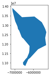
The alpha shape will be generated in the coordinate frame the geodataframe is in. In this example, we will project into an Albers Equal Area projection, construct our alpha shape in that coordinate system, and then convert back to the source projection.
import cartopy.crs as ccrs
gdf_proj = gdf.to_crs(ccrs.AlbersEqualArea().proj4_init)
gdf_proj.plot()
import alphashape
alpha_shape = alphashape.alphashape(gdf_proj)
alpha_shape.plot()
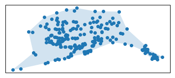
import matplotlib.pyplot as plt
ax = plt.axes(projection=ccrs.PlateCarree())
ax.scatter([p.x for p in gdf_proj['geometry']],
           [p.y for p in gdf_proj['geometry']],
           transform=ccrs.AlbersEqualArea())
ax.add_geometries(
    alpha_shape['geometry'],
    crs=ccrs.AlbersEqualArea(), alpha=.2)
plt.show()
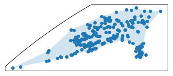
import matplotlib.pyplot as plt
ax = plt.axes(projection=ccrs.Robinson())
ax.scatter([p.x for p in gdf_proj['geometry']],
           [p.y for p in gdf_proj['geometry']],
           transform=ccrs.AlbersEqualArea())
ax.add_geometries(
    alpha_shape['geometry'],
    crs=ccrs.AlbersEqualArea(), alpha=.2)
plt.show()
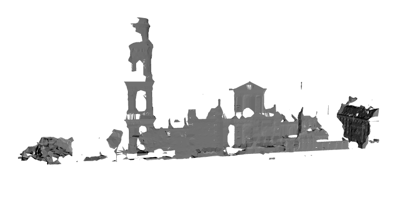
St. Sulpice Point Cloud Data
The following data can be obtained from the Lib E57 example data set found at the link below. To reduce the amount of data included in the alphashape toolbox repository, only a subset of point data was converted to a shapefile format and all data except point locations were dropped.
http://www.libe57.org/data.html

import os
import geopandas
data = os.path.join(os.getcwd(), 'data', 'Trimble_StSulpice-Cloud-50mm.shp')
gdf = geopandas.read_file(data)
from alphashape import alphashape
alphashape([point.coords[0] for point in gdf['geometry'][0]], 0.7).show()
Credits
This package was created with Cookiecutter and the audreyr/cookiecutter-pypackage project template.